
Principal Component Analysis Series-1
After a few more months of procrastination, here is Part 1 of my PCA series. I’m not an expert—just a curious learner sharing thoughts on a topic that has always felt a bit magical to me. Back at IIIT Delhi I studied PCA and still everytime I learn something new around it. Even today, I’m still figuring things out. Writing this blog helps me make sense of what I’m learning and, hopefully, get a little better at it along the way
How did one of the most powerful statistical techniques actually come to be? 🤔
The Origins
Here’s something fascinating: most statistical methods have murky origins, but PCA is different; it can be traced exactly where it came from or say it was conceptualized.
Two brilliant minds, 32 years apart, walking different paths toward the same underlying truth.
Pearson (1901) → Geometric intuition: “How do we fit a line (or plane) to a cloud of points?”
Hotelling (1933) → Algebraic formalization: principal components that successively maximize variance
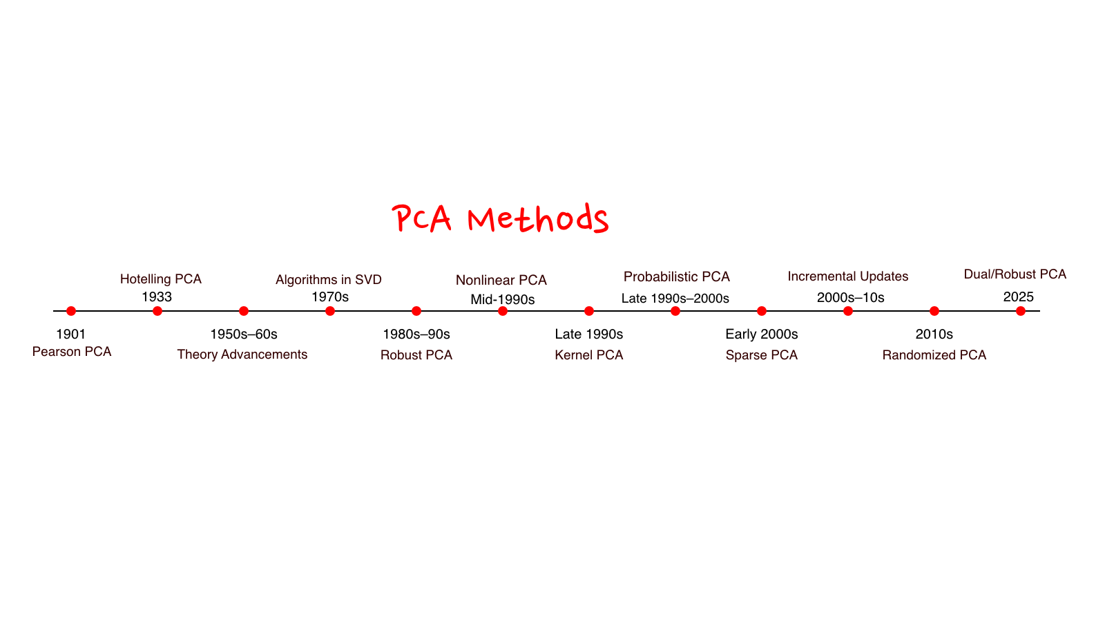
Below is a timeline of PCA research. I had a lot of fun putting this together and revisiting the ideas and mathematics behind many of these methods. If something catches your interest, feel free to explore it further, or reach out. I’m always happy to talk
Pearson’s Geometric Vision (1901)
Karl Pearson (1857–1936): the man who saw geometry in data.
The Core Insight
Pearson wasn’t thinking about “dimensionality reduction” (we’ll return to that in the next article). He asked a simpler question: What line best captures a cloud of points?
Imagine taking a group photo. You adjust their position until everyone fits naturally in the frame. That instinctive choice, capturing the widest spread was Pearson’s intuition.
A glimpse of the math (more in the next article)
I’ll share a bit of the mathematics here, but I’ll go deeper and more carefully in the next article.
At its core, Pearson was trying to answer a geometric question:
What single direction best represents a cloud of points?
Mathematically, we want to find a unit vector $\mathbf{u}$ that minimizes the squared distances from each data point to its projection onto that line. We can define the objective function:
$$ f(\mathbf{u}) = \sum_{i=1}^{n} \left| \mathbf{x}_i - (\mathbf{u}^\top \mathbf{x}_i)\mathbf{u} \right|^2 \quad \text{subject to } |\mathbf{u}| = 1 $$
This says: project each point onto a direction $\mathbf{u}$, measure how far the original point lies from that projection, and find the direction that minimizes the total error.
With a bit of algebra (which we’ll unpack later), this minimization is equivalent to a much cleaner maximization problem:
$$ f(\mathbf{u}) \equiv \mathbf{u}^\top \left( \sum_{i=1}^{n} \mathbf{x}_i \mathbf{x}_i^\top \right) \mathbf{u} $$
Takeaway: in 1D, the only principal component is along the line of the data. If you work out the formula you will eventualy end up capturing the variance of the distribution of the points. In higher dimensions, the challenge and the beauty of PCA lies in selecting the direction that maximizes variance among infinitely many possibilities.
A quiet optimism
Pearson famously wrote that these computations were “quite feasible” even for four or more variables.
Try computing the eigenvalues of a 10×10 matrix by hand, and you will quickly see why this was… optimistic.
Yet this is what makes his work remarkable. The mathematics (magic) was already there, clean, elegant, and conceptually complete. What was missing was computational power. PCA had to wait nearly six decades for computers to catch up with the idea.
Hotelling’s Algebraic Formulation (1933)
Harold Hotelling (1895–1973): the economist who formalized PCA
The Birth of “Principal Components”
Hotelling deliberately chose the term “components” (instead of “factors”) to avoid confusion with psychometric factor analysis. His key insight: principal components should capture successive contributions to total variance—the first component explains the maximum variance, the second explains the maximum remaining variance orthogonal to the first, and so on.
We can define an objective function $f(\mathbf{v})$ that measures the variance captured along a direction $\mathbf{v}$:
$$ f(\mathbf{v}) = \mathbf{v}^\top \Sigma \mathbf{v}, \quad \text{subject to } |\mathbf{v}| = 1 $$
Maximizing $f(\mathbf{v})$ gives the first principal component. The next component is found by maximizing the same function with the additional constraint that it is orthogonal to the previous components.
Mathematically, this is equivalent to solving the eigenvalue problem:
$$ \Sigma \mathbf{v}_i = \lambda_i \mathbf{v}_i $$
where $\lambda_1 \ge \lambda_2 \ge \dots \ge \lambda_p$ are the eigenvalues and $\mathbf{v}_i$ are the corresponding eigenvectors, which define the principal components.
The variance explained by the $i$-th principal component is:
$$ \text{Variance explained (PC $i$)} = \frac{\lambda_i}{\sum_{j=1}^{p} \lambda_j} $$
This is the formulation we teach today. In essence, Hotelling provided the computational recipe for PCA that connects the geometric intuition of Pearson to a clear algebraic solution.
Rao’s Extensions (1964)
C. R. Rao (1920–2023): the polymath who unified PCA theory. For those interested in Indian scientists’ contributions, Rao’s work is essential. His 1964 paper was a watershed moment: he explained PCA and connected it to many other methods.
What made Rao’s work important?
Three key contributions:
Theoretical unification
Showed PCA emerges from multiple perspectives:- Optimal low-rank matrix approximation.
- Maximum likelihood in specific models.
- Reconstruction error minimization.
Interpretational framework
Clarified what components mean:- How to interpret loadings.
- When to retain components,
- Mathematical vs. substantive significance.
Extensions
Connected PCA to canonical correlation analysis, factor analysis, regression, and prediction.
PCA as Low-Rank Approximation
Rao emphasized that PCA can be viewed as a low-rank approximation of the original data. We can define a function $f(\mathbf{W})$ that measures the total reconstruction error:
$$ f(\mathbf{W}) = |\mathbf{X} - \mathbf{X}\mathbf{W}\mathbf{W}^T|_F^2 $$
The goal is to minimize this function, i.e., find the projection matrix $\mathbf{W}$ that best approximates the data in a lower-dimensional subspace.
This perspective unifies PCA with linear algebra and shows that it is more than just a statistical trick—it is a fundamental method for approximating high-dimensional data.
A Personal Connection
During my master’s at IIIT Delhi, one night while using the library, I discovered Ian Jolliffe’s book online on “Principal Component Analysis” and got hooked 📚. That moment shaped my statistical learning. Yet my amazing mentor Prof. Debarka Sengupta (quite validly) still says I need to get better with my statistical understanding 😅 (his way of saying: keep learning 🚀). Fun fact: he received one of India’s top science awards and you can check out his work on his website 🌟. Why this book? There are many books and videos, but Jolliffe’s text stuck with me because it focuses deeply only on PCA 🔍.
Later, I ran a hands-on PCA session in R—the workshop page is available at this link. You can watch the video directly on YouTube: Watch the PCA Workshop on YouTube
Curious about computational biology and want more?
Join me at BioCodeTalks for curated tutorials, discussions, and insights on computational biology research and coding!
P.S. I’ll be releasing something exciting on bananas over there soon—stay tuned! 🍌
The Computing Revolution
With advances in computing power and memory, PCA has become fast and routine. How the computation is implemented really matters—a topic I’ll cover in more detail in a future article.
For now, here’s a simple Python snippet to demonstrate PCA on a large dataset:
import numpy as np
import time
from sklearn.decomposition import PCA

# Modern cancer genomics dataset
n_samples = 500
n_genes = 20000

X = np.random.randn(n_samples, n_genes)

start = time.time()
pca = PCA(n_components=50)
X_transformed = pca.fit_transform(X)
elapsed = time.time() - start

print(f"⚡ PCA on {n_genes:,} genes: {elapsed:.2f} seconds")
print(f"📊 Variance explained: {sum(pca.explained_variance_ratio_)*100:.1f}%")
Output:
⚡ PCA on 20,000 genes: 2.73 seconds
📊 Variance explained: 68.3%
Key Takeaways
What I covered in this post:
1901 — Pearson 🎨
Geometric intuition: fitting lines to point clouds
1933 — Hotelling 🔬
Algebraic formalization: “principal components” born
1964 — Rao 🌟
Theoretical unification: connecting PCA to broader statistics
Coming Up in This Series
This is just Part 1, we’ve covered a bit of history. Next:
- Part 2: Mathematical deep dive — eigenvectors, covariance matrices, optimization
- Part 3: Hands-on implementation — building PCA from scratch
- Part 4: Advanced extensions — Sparse PCA, Kernel PCA, Probabilistic PCA, Robust PCA
- Part 5: Biology applications — scRNA-seq, GWAS, proteomics
Some References
- Pearson (1901) — “On lines and planes of closest fit to systems of points in space”
- Hotelling (1933) — “Analysis of a complex of statistical variables into principal components”
- Rao (1964) — “The use and interpretation of principal component analysis in applied research”
- Jolliffe (1986, 2002, 2016) — Principal Component Analysis (all editions)
- Jolliffe & Cadima (2016) — “Principal component analysis: a review and recent developments”
- Ringnér (2008) — “What is principal component analysis?” (Nature Biotechnology)
- Lever et al. (2017) — “Principal component analysis” (Nature Methods)
🙏 Thank you for reading!
If you spot any errors or have suggestions, please reach out so I can update the post. Give hearts buy clicking heart at end.
📧 Drop me an email for chit chat about science or need mentorship etc at [email protected]
Acknowledgments: This post stands on the shoulders of Pearson, Hotelling, Rao, Jolliffe, and many others. I apologize for any omissions or mistakes.
Note: Some images in this post were generated using ChatGPT; the writing process was supported by Grammarly and other AI tools.